Offer Acceptance in the Freight Industry

Radu Manea, Benson Duong, Keagan Benson, and Nima Yazdani

Introduction

Flock Freight (FF) deals with different carriers and shipments, acting as a marketplace for freight carriers to place bids on shipping orders needed to be fulfilled, which is otherwise known as a freight broker

1. A Company X needs to ship an Order to a given place by a given time, but lack their own delivery vehicles.
2. Carriers are entities that offer delivery services.
3. FF is the intermediary between 1 and 2 above: One-by-one, FF processes an incoming stream of N offers from different carriers to deliver the order.
   • Only one offer will have the cheapest delivery rate rate ^t
   • FF cannot accidentally reject this offer (there's no going back when FF rejects an offer!)

Data Description

The full dataset includes 2 tables which contain: A) the orders, and descriptive information about it (Order Time, Pickup Deadline, accommodating conditions for its mode of delivery such as transport mode, refrigeration, and hazardness, etc); B) The offers by carriers to deliver said orders - this would be a many-to-one relationship, with the reference number column (assuming it’s a singleton list) being the foreign key. The offers table includes mostly information such as the rate of the offer, whether it is pooled or not, whether it was selected, and whether it was uncovered. We also created a supplemental dataset that maps 3 digit zip code identifiers to latitude and longitude coordinates.

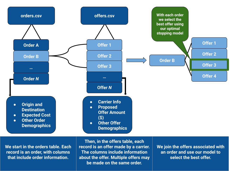
Flock Freight and The Offer Acceptance Problem

Our Model Approach

The model will comprise of 3 sub-models that together are used in a classification model that decides on whether an offer is acceptable or not, for a given order.

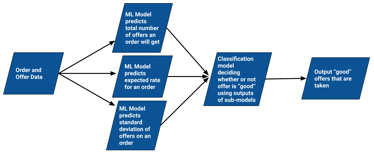
Number of Offers Prediction Model

The model takes in given order and estimates the number of offers that the order will receive.

Method: Use order characteristics such as estimated cost, pickup and dropoff location, distance apart, size of load and truck requirements to predict the number of offers that order will receieve.

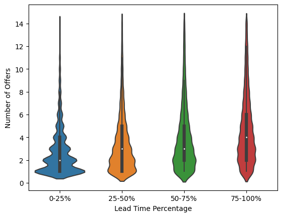
Problem: A noteable number of offers are accepted very early into the lead time. This results in the number of offers not reflecting the true amount of offers Flock would recieve if they waited till the order experied.

Solution: Weight the samples by precent into lead time when the offer was accepted. This allowed samples that were accepted further into the lead time to matter more when training the model.

Result: Acheived a mean absolute error of 2.68. This was 10.2% better than our baseline model and 6.5% better than our non-sample weighted model.

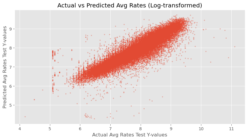
Rate Average Prediction Model

A model that takes in given order data and estimates the average of the rates of the offers that the order will receive

Method: Linear Regression

Results: Correlation of 85% between Predicted and Actual

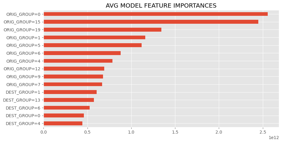
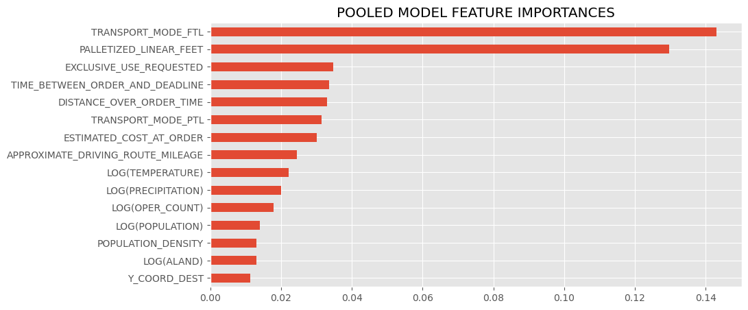
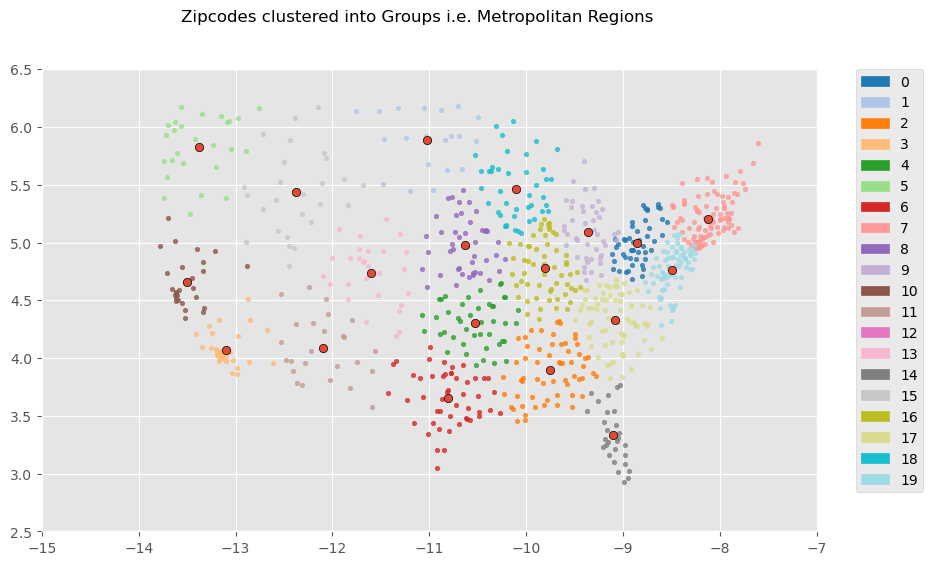
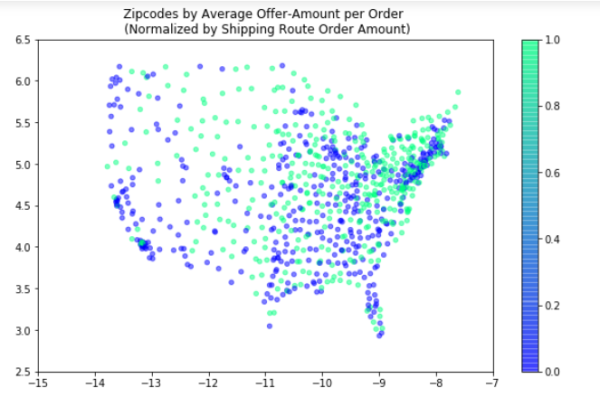
These are the most influential features of the avg model, either strongest in positive or negative correlation or otherwise determined by the model. Categorical features follow the format "FEATURE=CLASS", so "DEST_GROUP=4" would mean order with a destination zipcode closest to region 4 (see the regions cluster map in findings to see what group numbers correspond to which regions).

Rate Standard Deviation Prediction Model

A model that takes in given order data and estimates the standard deviation of the rates of the offers that the order will receive

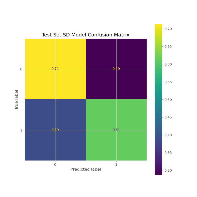
Method: Ordinalize as a binary classification ("low" StDev is 0, "high" is the median StDev), and applied Random Forest Classification for 2 classes

Results: ROC AUC Score of 65-68%

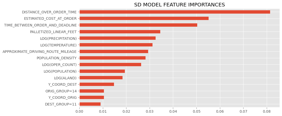
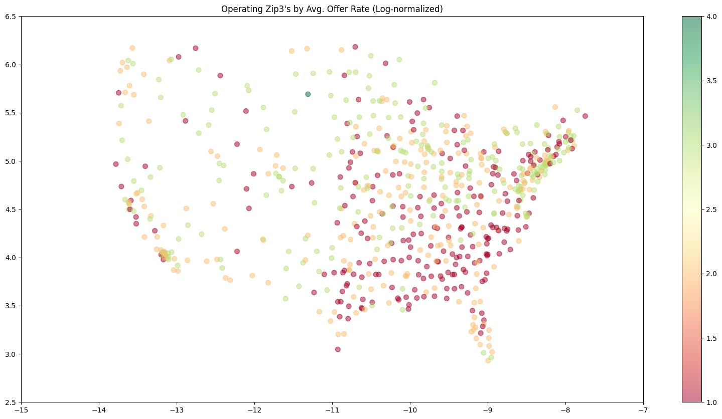
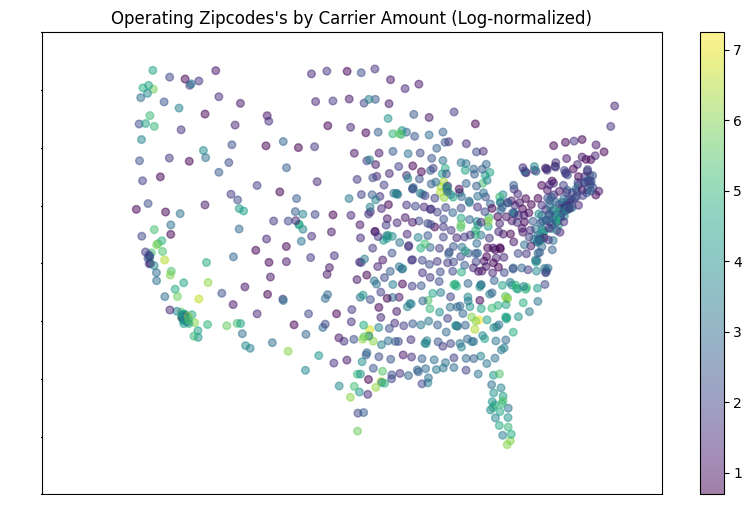
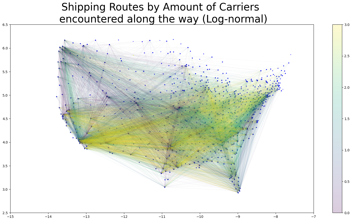
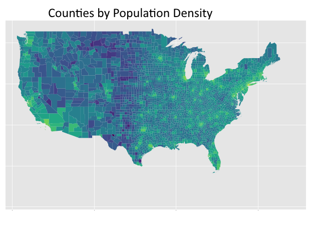
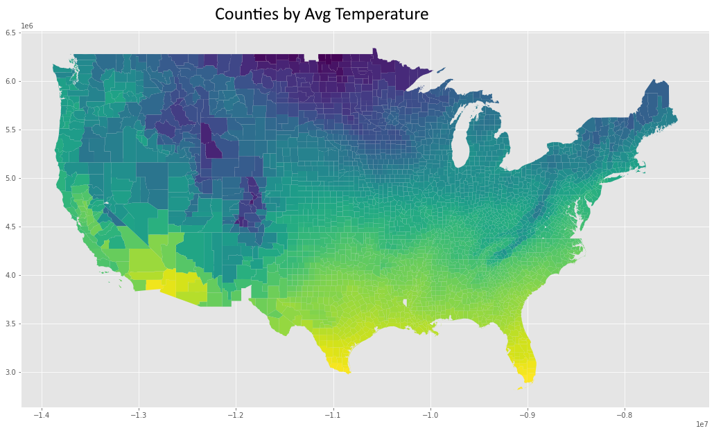
These are the most influential features of the st dev submodel, and in terms of a line drawn between the destination and origin, the average of population density, logged land area (see LOG(ALAND)), population, and logged temperature and precipitation of the encountered counties during the months of the order, and the (logged) amount of operating zipcode carriers encountered along the way (LOG(OPER_COUNT)), and information about proximity of the order's origin zipcode to regions (again, refer to the regions cluster map at the bottom)

Pooling Classification Model

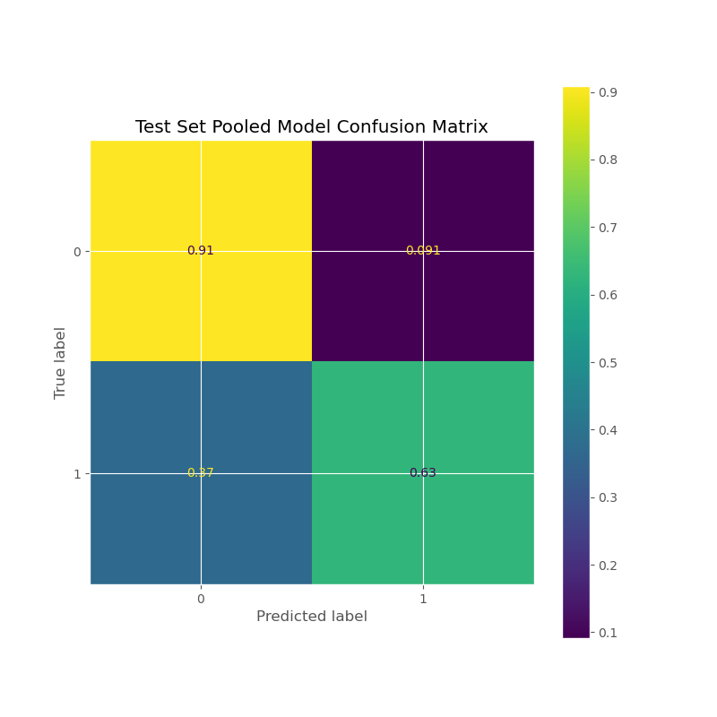
An optional model that takes in given order data and classifies on whether or not the order will receive (at any point) an offer in which it needs to be pooled. This pooling model is optional in that if its predictions are used as an extra feature for the standard deviation model, then it's been observed that the standard deviation model's accuracy will boost from 67% to 70%

Method: Logistic Regression; if for a given order, it receives offers where more than half of is pooled, it is classified as Yes

Results: ROC AUC Score of 80%

Findings and Results

Conclusion

• Our resulting offer acceptance model consists of a classifer which determines whether an offer is a good offer.
• We classified good offers as offers which flock freight accepted and the offers which had the lowest cost of their order.
• The features the logistic regression model was trained on were the offer rate and the outputs of the submodels; the estimated number of offers, the estimated cost and the estimated standard deviation.
• Our final model was able to select offers with an average price 4.44% lower than what Flock Freight had selected.